
티스토리 뷰
이번 글에서는 DBSCAN을 사용하여 데이터셋을 클러스터링하는 방법을 알아보겠습니다. DBSCAN은 Density-Based Spatial Clustering of Applications with Noise의 약자로, 밀도를 기반으로 하는 클러스터링 알고리즘입니다.
출처: https://github.com/chriswernst/
우선, 필요한 라이브러리를 불러오겠습니다. 코드에서는 numpy, matplotlib.pyplot, cv2, sklearn.cluster 패키지에서 DBSCAN을 사용합니다.
참고로 import cv2를 하기위해서는 opencv-python 패키지를 설치해야합니다.
import numpy as np
import matplotlib.pyplot as plt
import cv2
from sklearn.cluster import DBSCAN
다음으로, cluster_gen() 함수를 정의합니다. 이 함수는 n_clusters(클러스터의 개수), pts_minmax(클러스터 당 포인트의 범위), x_mult(y_mult)(클러스터 크기 조절을 위한 배수 범위), x_off(y_off)(클러스터 위치 오프셋 범위)와 같은 여러 매개변수를 받아들입니다.
def cluster_gen(n_clusters, pts_minmax=(10, 100), x_mult=(1, 4), y_mult=(1, 3),
                x_off=(0, 50), y_off=(0, 50)):

    # n_clusters = number of clusters to generate
    # pts_minmax = range of number of points per cluster
    # x_mult = range of multiplier to modify the size of cluster in the x-direction
    # y_mult = range of multiplier to modify the size of cluster in the x-direction
    # x_off = range of cluster position offset in the x-direction
    # y_off = range of cluster position offset in the y-direction

    # Initialize some empty lists to receive cluster member positions
    clusters_x = []
    clusters_y = []
    # Genereate random values given parameter ranges
    n_points = np.random.randint(pts_minmax[0], pts_minmax[1], n_clusters)
    x_multipliers = np.random.randint(x_mult[0], x_mult[1], n_clusters)
    y_multipliers = np.random.randint(y_mult[0], y_mult[1], n_clusters)
    x_offsets = np.random.randint(x_off[0], x_off[1], n_clusters)
    y_offsets = np.random.randint(y_off[0], y_off[1], n_clusters)

    # Generate random clusters given parameter values
    for idx, npts in enumerate(n_points):

        xpts = np.random.randn(npts) * x_multipliers[idx] + x_offsets[idx]
        ypts = np.random.randn(npts) * y_multipliers[idx] + y_offsets[idx]
        clusters_x.append(xpts)
        clusters_y.append(ypts)

    # Return cluster positions
    return clusters_x, clusters_y
이제 cluster_gen() 함수를 사용하여 n_clusters 개수의 클러스터를 생성하고, 생성된 클러스터를 OpenCV 형식의 데이터셋으로 변환합니다.
n_clusters = 50
clusters_x, clusters_y = cluster_gen(n_clusters)
# Convert to a single dataset in OpenCV format
data = np.float32((np.concatenate(clusters_x), np.concatenate(clusters_y))).transpose()
다음으로, DBSCAN을 사용하여 클러스터링을 수행합니다. DBSCAN() 함수는 두 개의 결과를 반환합니다. 첫 번째는 각 포인트에 할당된 클러스터 레이블을 포함하는 배열이고, 두 번째는 클러스터링에서 핵심 포인트를 나타내는 마스크입니다.
# Define max_distance (eps parameter in DBSCAN())
max_distance = 1
db = DBSCAN(eps=max_distance, min_samples=10).fit(data)

# Extract a mask of core cluster members
core_samples_mask = np.zeros_like(db.labels_, dtype=bool)
core_samples_mask[db.core_sample_indices_] = True

# Extract labels (-1 is used for outliers)
labels = db.labels_
n_clusters = len(set(labels)) - (1 if -1 in labels else 0)
unique_labels = set(labels)
마지막으로, 원래 데이터와 클러스터링된 결과를 시각화하기 위해 matplotlib을 사용합니다. subplot() 함수를 사용하여 두 개의 서브 플롯을 생성하고, plot() 함수를 사용하여 데이터 포인트를 그립니다. 또한, 클러스터링 결과를 나타내기 위해 unique_labels를 사용하여 각 클러스터에 색상을 지정하고, 핵심 포인트, 가장자리 포인트, 그리고 이상치에 대해 다른 마커 스타일과 크기를 사용하여 시각적으로 나타냅니다. 클러스터의 수를 제목에 표시합니다.
min_x = np.min(data[:, 0])
max_x = np.max(data[:, 0])
min_y = np.min(data[:, 1])
max_y = np.max(data[:, 1])

fig = plt.figure(figsize=(12,6))
plt.subplot(121)
plt.plot(data[:,0], data[:,1], 'ko')
plt.xlim(min_x, max_x)
plt.ylim(min_y, max_y)
plt.title('Original Data', fontsize = 20)

plt.subplot(122)
# The following is just a fancy way of plotting core, edge and outliers
# Credit to: http://scikit-learn.org/stable/auto_examples/cluster/plot_dbscan.html#sphx-glr-auto-examples-cluster-plot-dbscan-py
colors = [plt.cm.Spectral(each) for each in np.linspace(0, 1, len(unique_labels))]
for k, col in zip(unique_labels, colors):
    if k == -1:
        # Black used for noise.
        col = [0, 0, 0, 1]

    class_member_mask = (labels == k)

    xy = data[class_member_mask & core_samples_mask]
    plt.plot(xy[:, 0], xy[:, 1], 'o', markerfacecolor=tuple(col),
             markeredgecolor='k', markersize=7)

    xy = data[class_member_mask & ~core_samples_mask]
    plt.plot(xy[:, 0], xy[:, 1], 'o', markerfacecolor=tuple(col),
             markeredgecolor='k', markersize=3)
plt.xlim(min_x, max_x)
plt.ylim(min_y, max_y)
plt.title('DBSCAN: %d clusters found' % n_clusters, fontsize = 20)
fig.tight_layout()
plt.subplots_adjust(left=0.03, right=0.98, top=0.9, bottom=0.
matplotlib의 tight_layout() 함수를 사용하여 플롯 요소들을 자동으로 조정하고, subplots_adjust() 함수를 사용하여 서브 플롯 간의 간격을 조정합니다.
이제 전체 코드를 살펴보겠습니다.
import numpy as np
import matplotlib.pyplot as plt
import cv2
from sklearn.cluster import DBSCAN


# Define a function to generate clusters
def cluster_gen(n_clusters, pts_minmax=(10, 100), x_mult=(1, 4), y_mult=(1, 3),
                x_off=(0, 50), y_off=(0, 50)):

    # n_clusters = number of clusters to generate
    # pts_minmax = range of number of points per cluster
    # x_mult = range of multiplier to modify the size of cluster in the x-direction
    # y_mult = range of multiplier to modify the size of cluster in the x-direction
    # x_off = range of cluster position offset in the x-direction
    # y_off = range of cluster position offset in the y-direction

    # Initialize some empty lists to receive cluster member positions
    clusters_x = []
    clusters_y = []
    # Generate random values given parameter ranges
    n_points = np.random.randint(pts_minmax[0], pts_minmax[1], n_clusters)
    x_multipliers = np.random.randint(x_mult[0], x_mult[1], n_clusters)
    y_multipliers = np.random.randint(y_mult[0], y_mult[1], n_clusters)
    x_offsets = np.random.randint(x_off[0], x_off[1], n_clusters)
    y_offsets = np.random.randint(y_off[0], y_off[1], n_clusters)

    # Generate random clusters given parameter values
    for idx, npts in enumerate(n_points):
        xpts = np.random.randn(npts) * x_multipliers[idx] + x_offsets[idx]
        ypts = np.random.randn(npts) * y_multipliers[idx] + y_offsets[idx]
        clusters_x.append(xpts)
        clusters_y.append(ypts)

    # Return cluster positions
    return clusters_x, clusters_y


# Generate some clusters!
n_clusters = 50
clusters_x, clusters_y = cluster_gen(n_clusters)

# Convert to a single dataset in OpenCV format
data = np.float32((np.concatenate(clusters_x), np.concatenate(clusters_y))).transpose()

# Define max_distance (eps parameter in DBSCAN())
max_distance = 1
db = DBSCAN(eps=max_distance, min_samples=10).fit(data)

# Extract a mask of core cluster members
core_samples_mask = np.zeros_like(db.labels_, dtype=bool)
core_samples_mask[db.core_sample_indices_] = True

# Extract labels (-1 is used for outliers)
labels = db.labels_
n_clusters = len(set(labels)) - (1 if -1 in labels else 0)
unique_labels = set(labels)

# Plot up the results!
min_x = np.min(data[:, 0])
max_x = np.max(data[:, 0])
min_y = np.min(data[:, 1])
max_y = np.max(data[:, 1])

fig = plt.figure(figsize=(12,6))
plt.subplot(121)
plt.plot(data[:,0], data[:,1], 'ko')
plt.xlim(min_x, max_x)
plt.ylim(min_y, max_y)
plt.title('Original Data', fontsize = 20)

plt.subplot(122)
# The following is just a fancy way of plotting core, edge and outliers
# Credit to: http://
분류분석 결과를 plot합니다.
plt.subplot(122)
# The following is just a fancy way of plotting core, edge and outliers
# Credit to: http://scikit-learn.org/stable/auto_examples/cluster/plot_dbscan.html#sphx-glr-auto-examples-cluster-plot-dbscan-py
colors = [plt.cm.Spectral(each) for each in np.linspace(0, 1, len(unique_labels))]
for k, col in zip(unique_labels, colors):
    if k == -1:
        # Black used for noise.
        col = [0, 0, 0, 1]

    class_member_mask = (labels == k)

    xy = data[class_member_mask & core_samples_mask]
    plt.plot(xy[:, 0], xy[:, 1], 'o', markerfacecolor=tuple(col),
             markeredgecolor='k', markersize=7)

    xy = data[class_member_mask & ~core_samples_mask]
    plt.plot(xy[:, 0], xy[:, 1], 'o', markerfacecolor=tuple(col),
             markeredgecolor='k', markersize=3)
plt.xlim(min_x, max_x)
plt.ylim(min_y, max_y)
plt.title('DBSCAN: %d clusters found' % n_clusters, fontsize = 20)
fig.tight_layout()
plt.subplots_adjust(left=0.03, right=0.98, top=0.9, bottom=0.05)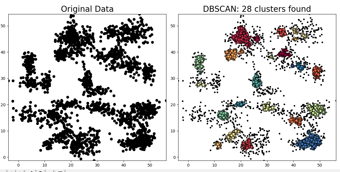
'머신러닝 파이썬' 카테고리의 다른 글
| 선형 회귀를 이용한 시계열 예측의 한계와 대안적인 방법(python) (0) | 2023.03.17 |
|---|---|
| 시계열 데이터 분석: Pandas를 이용한 자기상관 플롯(Autocorrelation Plot) (0) | 2023.03.17 |
| 시계열의 stationarity 를 검정하는 ADF test 예시(파이썬) (0) | 2023.03.16 |
| python에서 dropna() 또는 fillna() 를 이용한 결측치 메우기 (0) | 2023.03.14 |
| 계층적 군집화로 iris 데이터 분석하기(병합적 군집화) (0) | 2023.03.07 |